Unlock insights from your time series data with our expert guide to EDA techniques. Learn how to visualize trends, detect anomalies, and prepare your data for modeling. Boost your data science skills today!
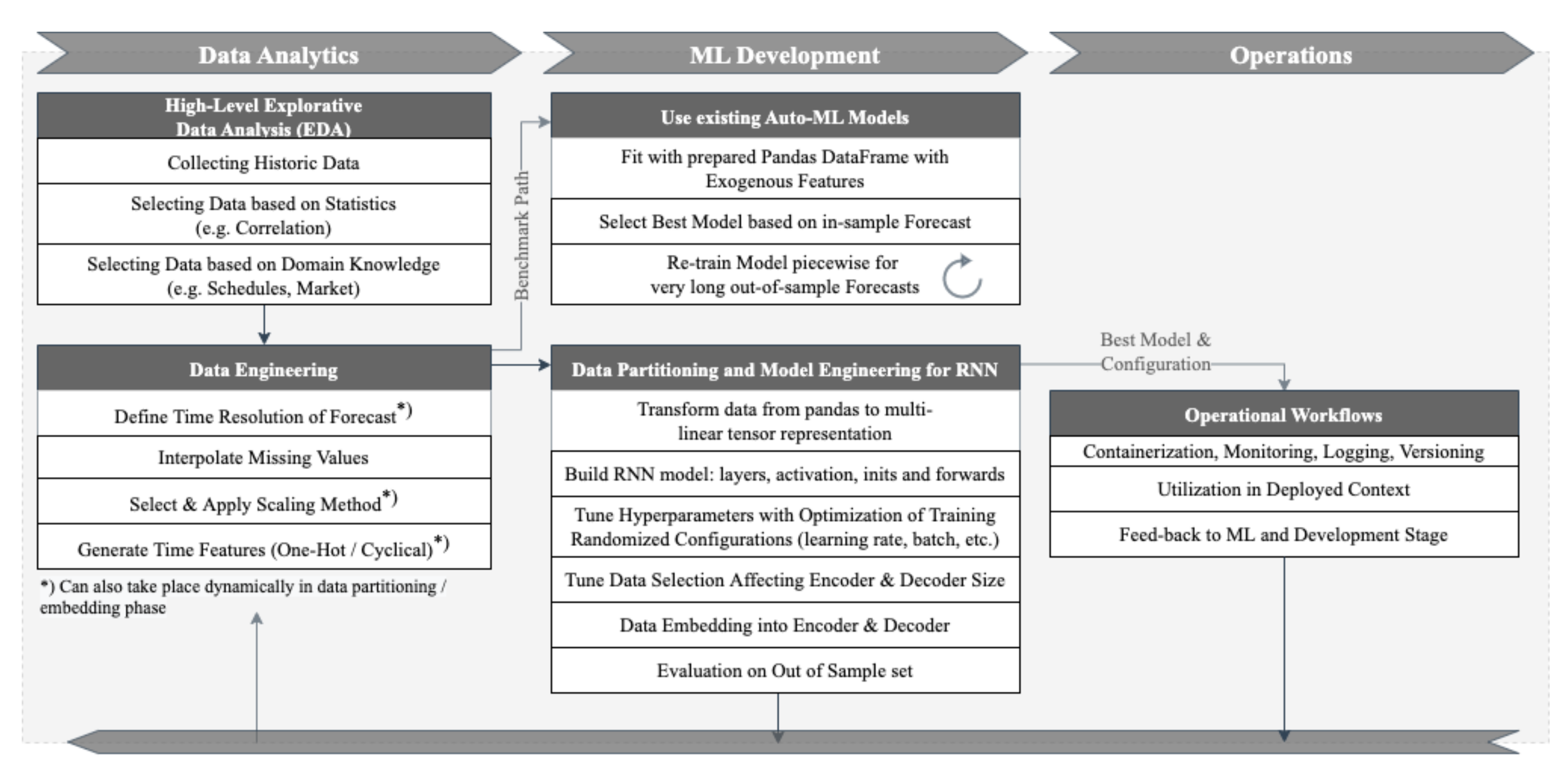
By utilizing exploratory data analysis techniques such as plotting time series graphs, decomposing data, and identifying autocorrelation, analysts can gain valuable insights into the underlying patterns of the data. Effective EDA can lead to better forecasting models and decision-making processes based on historical data trends.
Understanding the behavior of time series data through EDA is crucial for businesses looking to make informed strategic decisions and predictions based on past performance.
Introduction To Time Series Data
Time series data is data collected over time. It records the same variable at different points. This type of data is unique and valuable. It helps us understand trends and patterns.
Importance In Various Fields
Time series data is crucial in many fields. Here are some examples:
- Finance: Stock prices, exchange rates, and market trends.
- Healthcare: Patient vital signs, disease spread, and treatment outcomes.
- Weather: Temperature, rainfall, and storm tracking.
- Economics: GDP, unemployment rates, and inflation.
Each field uses time series data to make decisions. It helps predict future events. This makes it a powerful tool.
Challenges In Analysis
Analyzing time series data comes with challenges. Here are some common ones:
- Trends: Long-term changes in the data.
- Seasonality: Regular patterns that repeat over time.
- Noise: Random variations in the data.
- Missing Values: Gaps in the data that need filling.
Each challenge requires different techniques. Handling them well is key to accurate analysis.
Understanding these challenges helps improve analysis. Proper techniques lead to better insights.
Credit: towardsdatascience.com
Basic Eda Techniques
Exploratory Data Analysis (EDA) is essential for understanding time series data. Basic EDA techniques help uncover patterns, detect anomalies, and prepare data for further analysis. These steps are foundational for any time series project.
Data Cleaning
Data cleaning is the first step in EDA. It ensures the data is accurate and usable. This process removes errors, inconsistencies, and irrelevant information. Clean data provides reliable insights.
Here are some common data cleaning tasks:
- Removing duplicate entries
- Correcting errors in data
- Standardizing data formats
Handling Missing Values
Missing values are common in time series data. They can distort analysis results. Handling them correctly is crucial.
There are several ways to handle missing values:
- Deletion: Remove rows or columns with missing values. This is simple but can lead to data loss.
- Imputation: Replace missing values with estimates. Common methods include mean, median, or mode imputation.
- Interpolation: Use surrounding values to estimate missing ones. Linear interpolation is a popular choice.
Here’s an example of filling missing values using Python:
import pandas as pd
data = {'date': ['2023-01-01', '2023-01-02', '2023-01-03', '2023-01-05'],
        'value': [10, None, 15, 20]}
df = pd.DataFrame(data)
df['value'] = df['value'].interpolate()
print(df)
This code fills missing values using linear interpolation.
Visualizing Time Series Data
Visualizing time series data helps understand patterns and trends. Effective visualization techniques reveal insights otherwise hidden in raw data. This section covers popular methods for visualizing time series data.
Line Plots
Line plots are fundamental for time series visualization. They show data points connected by straight lines. This method is simple but effective. It highlights trends and patterns over time.
Here’s an example of a line plot:
import matplotlib.pyplot as plt

# Sample time series data
time = [1, 2, 3, 4, 5]
values = [10, 20, 15, 25, 30]

plt.plot(time, values)
plt.title('Line Plot Example')
plt.xlabel('Time')
plt.ylabel('Values')
plt.show()
The plot above shows changes in values over time. Notice the peaks and troughs. These indicate fluctuations in the data.
Seasonal Decomposition
Seasonal decomposition breaks down time series data into three components: trend, seasonality, and residuals. This method helps identify underlying patterns. The seasonal component shows repeating cycles. The trend component indicates overall direction. Residuals capture irregular variations.
Here’s an example of seasonal decomposition:
import pandas as pd
from statsmodels.tsa.seasonal import seasonal_decompose

# Sample time series data
data = {'Month': pd.date_range(start='1/1/2020', periods=12, freq='M'), 'Value': [10, 20, 15, 25, 30, 35, 40, 45, 50, 55, 60, 65]}
df = pd.DataFrame(data)
df.set_index('Month', inplace=True)

decomposition = seasonal_decompose(df['Value'], model='additive')

decomposition.plot()
plt.show()
The decomposition results in three plots. The first plot shows the original data. The second plot reveals the trend. The third plot displays the seasonal component. The fourth plot captures the residuals.

Credit: www.amazon.com
Trend Analysis
Trend analysis helps us understand the patterns in time series data. These patterns show how data changes over time. Understanding trends is crucial for forecasting and decision-making.
Identifying Trends
Identifying trends involves spotting the general direction of data points. These directions can be upward, downward, or flat. Visual tools like line plots are helpful for this purpose.
Line plots show data points connected by lines. This helps visualize trends clearly. Here is a simple example:
import matplotlib.pyplot as plt

# Sample data
time = [1, 2, 3, 4, 5]
values = [10, 12, 15, 18, 20]

# Create line plot
plt.plot(time, values)
plt.xlabel('Time')
plt.ylabel('Values')
plt.title('Line Plot of Time Series Data')
plt.show()
Smoothing Techniques
Smoothing techniques help remove noise from data. This makes trends easier to see. Common methods include moving averages and exponential smoothing.
Moving averages calculate the average of data points over a set period. This method smooths out short-term fluctuations.
import pandas as pd

# Sample data
data = {'time': [1, 2, 3, 4, 5], 'values': [10, 12, 15, 18, 20]}
df = pd.DataFrame(data)

# Calculate moving average
df['moving_average'] = df['values'].rolling(window=2).mean()
print(df)
Exponential smoothing gives more weight to recent data points. This method is useful for forecasting.
import statsmodels.api as sm

# Sample data
values = [10, 12, 15, 18, 20]

# Apply exponential smoothing
smoothed_values = sm.tsa.SimpleExpSmoothing(values).fit(smoothing_level=0.2).fittedvalues
print(smoothed_values)
Seasonal Patterns
Understanding seasonal patterns in time series data is crucial for accurate analysis. Seasonality refers to periodic fluctuations that repeat over a specific period. These patterns can significantly affect forecasting and other analytical processes.
Detecting Seasonality
Detecting seasonality involves identifying regular intervals of recurring events. Common methods to detect seasonality include:
- Visual Inspection: Plot the data to identify repeating patterns visually.
- Autocorrelation Function (ACF): Check for significant correlations at specific lags.
- Seasonal Decomposition: Decompose the time series into trend, seasonal, and residual components using methods like STL (Seasonal and Trend decomposition using Loess).
Impact On Forecasting
Seasonal patterns significantly affect forecasting accuracy. Ignoring seasonality can lead to poor predictions. Key impacts include:
- Model Selection: Choose models that handle seasonality, like SARIMA or Holt-Winters.
- Parameter Tuning: Optimize model parameters to account for seasonal effects.
- Performance Metrics: Use metrics like RMSE or MAE to evaluate model performance with seasonality considered.
Incorporating seasonality ensures more accurate and reliable forecasts. This approach provides better decision-making insights.
Detecting Outliers
Outliers are data points that differ greatly from other observations. Detecting outliers is crucial. It helps understand data anomalies and improve model accuracy.
Methods For Outlier Detection
There are various methods to detect outliers in time series data. Below are some common techniques:
- Visualization: Plot the time series data. Look for points that stand out.
- Statistical Methods: Use Z-scores or IQR. They help identify extreme values.
- Machine Learning: Algorithms like Isolation Forest can detect outliers.
Visualization is the simplest method. It provides a clear view of anomalies. Statistical methods involve calculations but are effective. Machine learning methods are advanced and accurate.
Handling Outliers
After detecting outliers, the next step is handling them. Here are some techniques:
- Removal: Remove the outliers. This method is straightforward but risky.
- Transformation: Apply transformations like log or square root. It reduces the impact of outliers.
- Imputation: Replace outliers with mean or median values. This retains data integrity.
Removing outliers can simplify data but may lose information. Transformations help in reducing their effect. Imputation is useful for maintaining the dataset’s overall structure.
| Method | Pros | Cons |
|---|---|---|
| Removal | Simple and easy | Risk of losing data |
| Transformation | Reduces impact | May not always work |
| Imputation | Maintains integrity | Can introduce bias |
In summary, detecting and handling outliers is essential. It ensures the accuracy and reliability of your time series analysis.
Correlation Analysis
Correlation analysis helps identify relationships between time series variables, revealing patterns and dependencies. This EDA technique is crucial for understanding how different time points interact.
Correlation analysis is vital in understanding relationships between time series data.
Autocorrelation
Autocorrelation measures a variable’s correlation with itself over different time intervals. It helps in identifying repeating patterns in data.
Cross-correlation
Cross-correlation compares two different time series to identify relationships and patterns between them. It is useful in analyzing how one series affects another.

Credit: www.mdpi.com
Advanced Eda Techniques
Advanced EDA techniques unlock deep insights from time series data, revealing patterns and trends. Explore these methods to enhance predictive accuracy and data understanding.
Fourier Transform
Using Fourier Transform in time series data analysis reveals frequency components.
Wavelet Transform
Wavelet Transform is effective for analyzing data at different scales.
Advanced EDA Techniques offer deeper insights into time series data.
Fourier Transform breaks down a signal into its frequency components.
Wavelet Transform helps in analyzing data at varying resolutions.
Case Studies
Case studies offer practical insights into applying EDA techniques to time series data. They show real-world applications and the lessons learned from these implementations. This section delves into specific examples and the valuable knowledge gained.
Real-world Examples
Let’s explore some real-world examples where EDA techniques have been applied to time series data.
| Industry | Use Case | EDA Techniques |
|---|---|---|
| Finance | Stock Price Analysis | Line Plots, Moving Averages |
| Healthcare | Patient Monitoring | Time Series Decomposition, Seasonal Plots |
| Retail | Sales Forecasting | Histogram, Box Plots |
Lessons Learned
From these case studies, several lessons have emerged:
- Understand Data Structure: Knowing the data’s structure aids in selecting the right EDA techniques.
- Visualize Data: Visual representations like line plots and histograms make patterns clear.
- Handle Seasonality: Identifying seasonal trends helps in accurate forecasting.
- Use Decomposition: Decomposing time series data into trend, seasonality, and residuals reveals deeper insights.
By leveraging these lessons, you can enhance your analysis and make better data-driven decisions.
Frequently Asked Questions
What Are The Techniques Used In Eda For Time Series Analysis?
Techniques used in EDA for time series analysis include visualization, decomposition, autocorrelation, and stationarity tests. Visualization helps identify patterns and trends. Decomposition breaks down data into components. Autocorrelation checks for lag relationships. Stationarity tests determine if the series is stable over time.
What Are The Techniques Used In Eda?
EDA techniques include data visualization, summary statistics, correlation analysis, and data cleaning. Visualization tools like histograms and scatter plots reveal patterns. Summary statistics provide insights on central tendency and dispersion. Correlation analysis identifies relationships between variables, while data cleaning addresses missing values and outliers.
What Are The Techniques For Time Series Data?
Techniques for time series data include ARIMA, Exponential Smoothing, Seasonal Decomposition, and LSTM models. Use these for forecasting trends.
What Are The 5 Time Series Forecasting Methods?
The 5 time series forecasting methods are: 1. ARIMA (Auto-Regressive Integrated Moving Average) 2. Exponential Smoothing (ETS) 3. Seasonal Decomposition of Time Series (STL) 4. Prophet 5. Long Short-Term Memory (LSTM) Networks
Conclusion
Mastering EDA techniques for time series data is essential. These techniques help uncover valuable insights and trends. Implementing them can significantly improve forecasting accuracy. Stay updated with new tools and methods to enhance your analysis. Start applying these techniques today and see the difference they make in your data-driven decisions.


